An Alternative Traffic Speed-Density Relationship

Previously we've examined a macroscopic traffic model, which contained, as one of its model equations, a relationship between speed and density. That relationship is reproduced here:
$$v = v_f (1 - \rho/\rho_j),$$ where
\(v\) = vehicle speed (m/s);
\(v_f\) = free flow speed (m/s);
\(\rho\) = vehicular density (veh/m); and
\(\rho_j\) = jam density (veh/m), the average vehicles per metre in stationary traffic.

Here I present an alternative speed-density relationship based on headways. Headway is the spacing between vehicles, usually as a time, but it can also be expressed in terms of distance.

In addition to expressing the above headway concepts, the new speed equation should satisfy two conditions. At zero density, the speed should be \(v_f\), and at the jam density, the speed should be zero.

But first we will develop the headway concept. As stated above, headway is usually expressed as a time. That's a good starting point. If we denote temporal headway as \(h_t\) (s/veh), then we may write that: $$h_t = 1/q = 1/\rho v,$$ or rearranged: $$v = 1/\rho h_t.$$ There is a difficulty with that relationship because at the jam density, the speed is still non-zero. However, note that \(1/\rho\) is the distance per vehicle. If we replace \(1/\rho\) with \(1/\rho-1/\rho_j\), then the equation becomes: $$v = \frac{1}{h_t}(1/\rho-1/\rho_j),$$ and the speed at the jam density is zero.

The only issue left with the above equation is that the speed is undefined at zero density, instead of being \(v_f\). To overcome this and ensure that the speed is \(v_f\) at zero density, I've developed this equation: $$v = \frac{1}{\frac{1}{v_f} + \frac{h_t}{(1/\rho-1/\rho_j)}}.$$ Unfortunately it still suffers from being undefined at zero density, but it's now more easily overcome. The final formula for speed is: $$v = \frac{1}{\frac{1}{v_f} + \frac{h_t\rho}{(1-\rho/\rho_j)}}.$$

We have previously analysed the original flow-density relationship, and we will do similar here. Thanks the the equation \(q=\rho v\), in this alternative formulation, flow is given by: $$q = \frac{\rho}{\frac{1}{v_f} + \frac{h_t\rho}{(1-\rho/\rho_j)}}.$$
The analysis to determine capacity for this relationship is more involved, but definitely solvable. The critical density is given by: $$\rho_c = \frac{1-\sqrt{h_t v_f \rho_j}}{1/\rho_j - v_f h_t}.$$ Capacity may be calculated by using the critical density in the flow equation above. The relationships are displayed in this graph for \(\rho_j\) = 1/7 veh/m and \(h_t\) = 0.7 s/veh:

An alternative flow-density relationship based on headways.

Interestingly, the original flow-density relationship is approximately recovered when \(h_t\) = 1/4 s/veh. That is encouraging, and means that this alternative speed-density relationship might be considered as a generalisation of the original one. But why is it the specific value of \(h_t\) = 1/4 s/veh? Well, after some rearranging of the final speed formula above, we can write it as: $$v = \frac{v_f (1-\rho/\rho_j)}{1+\rho(h_t v_f - 1/\rho_j)}.$$ The top part happens to be equal to our original speed equation, so to make them completely equal, we just have to satisfy \(h_t v_f = 1/\rho_j\). Finally, if \(v_f\) = 27.78 m/s (100 km/h), and \(\rho_j\) = 1/7 veh/m, then \(h_t\) should be 0.252 s. No wonder a headway of 0.25 s appeared to give the original speed-density relationship.

Discretising Base Traffic Model Equations

This post is a followup of these earlier posts. Here we discretise the traffic model equations to let us solve them numerically. Here are the model equations (including boundary conditions) all together in one place:
$$q = \rho v,$$ $$\frac{\partial \rho}{\partial t} + \frac{\partial q}{\partial x} = S(x,t),$$ $$v=v_f ( 1 - \rho/\rho_j ),$$ $$S(x,t) = 0,$$ $$\rho(x,0) = 0,$$ and $$\rho(0,t) = \rho_j/4.$$ where
\(q\) = traffic flow rate (veh/s) past the point;
\(\rho\) = vehicular density (veh/m);
\(v\) = vehicle speed (m/s);
\(\partial\) indicates partial differentiation;
\(t\) = time (s);
\(x\) = distance (m) along road;
\(S\) = vehicles entering (+ve) or leaving (-ve) the road (veh/m/hr);
\(v_f\) = free flow speed (m/s); and
\(\rho_j\) = jam density (veh/m), the average vehicles per metre in stationary traffic.

Note that we've set \(S(x,t)\) to zero. This means that no vehicles are leaving or entering the road apart from at the ends.

The presence of the very simple equation for flow, \(q\), means that we can eliminate flow from the equations altogether. When a value for flow is needed, we can just multiply density and speed together. As we progress, we may (or may not) find it desirable to do the same with speed. With flow removed, the main equation becomes: $$\frac{\partial \rho}{\partial t} + \frac{\partial \rho v}{\partial x} = S(x,t).$$ My favourite discretisation method is to use control volumes - the finite volume method. The first step is to divide the domain into cells, or control volumes. Here is how we will do that:

Discretisation grid for our traffic equations, showing coordinates for cells 1, i and n.

where a trailing minus sign indicates the left boundary, and a trailing plus sign indicates the right boundary. Because the right boundary of one cell is the left boundary of the next cell, we have \(x_{i+} = x_{i+1-}\). Dots indicate the location used to calculate representative model values contents for each cell.

There is also a time dimension, and we'll refer to the current time with \(t_c\), the target, or future, time with \(t_f\). The time step of our discretisation is given by \(t_f - t_c = \Delta t\).

We will discretise our density equation by integrating it over the volume of each cell, 1 to \(n\). Since we have two dimension, \(x\) and \(t\), the integration over the volume involves two integrals.

Body Cells: 2 to n-1

First we'll integrate over space: $$\int_{x_{i-}}^{x_{i+}}\frac{\partial \rho}{\partial t}\,dx + \int_{x_{i-}}^{x_{i+}}\frac{\partial \rho v}{\partial x}\,dx = 0.$$ The first integral is approximated using the rectangle rule with one rectangle using the midpoint approximation (\(x=x_i\)). The second integral simplifies thanks to the fundamental theorem of calculus. Applying those (and explicitly writing the function arguments for \(\rho\) and \(v\)), we get: $$(x_{i+}-x_{i-}) \frac{\partial \rho(x_i,t)}{\partial t} + \left[\rho(x,t) v(x,t)\right]_{x_{i-}}^{x_{i+}} = 0.$$ Now we'll apply the time integral from the current time, \(t_c\), to the future time, \(t_f\). For the second integral, we use the rectangle rule, with top left corner approximation (\(t=t_c\)): $$(x_{i+}-x_{i-}) \left[\rho(x_i,t)\right]_{t_c}^{t_f} + (t_f-t_c) \left[\rho(x,t_c) v(x,t_c)\right]_{x_{i-}}^{x_{i+}} = 0.$$ Next, we rearrange it to have the density at the future time on the left, and everything else on the right: $$\rho(x_i,t_f) = \rho(x_i,t_c) - \frac{t_f-t_c}{x_{i+}-x_{i-}}\left(\rho(x_{i+},t_c) v(x_{i+},t_c) - \rho(x_{i-},t_c) v(x_{i-},t_c)\right).$$

Left Boundary Cell: 1

The left boundary equation doesn't need to be obtained by integrating as it is given by the existing boundary condition: $$\rho(0,t) = \rho_j/4.$$

Right Boundary Cell: n

For the right boundary cell, we can reuse the equation from the body cells, but updated to refer to the last cell's coordinates (\(i\rightarrow n, x_{i+}\rightarrow x_{n}\)): $$\rho(x_n,t_f) = \rho(x_n,t_c) - \frac{t_f-t_c}{x_n-x_{n-}}\left(\rho(x_n,t_c) v(x_n,t_c) - \rho(x_{n-},t_c) v(x_{n-},t_c)\right).$$

The next step in this thread will be solving these discretised equations.

Smooth Minimum and Maximum

The functions we examine in this post are closely related to p-norms. Lets say we have two equations that describe aspects of a relationship. For example, we might describe the selling price of an item in terms of a discounted price, \(d\), for small purchases, and a lower bound price, \(u\), for bulk purchases. In that case, we might have two equations to describe price: $$d(x)=202-2x,$$ and $$u(x)=150,$$ where \(x\) is the number of units purchased in a single transaction. In this case, it might be fine to simply decide the selling price, \(p\) as $$p(x) = \max(d(x), u(x)),$$ but what if we want a formula for the selling price that has continuous derivatives? (i.e. is smooth) Well, the formula I found in an attempt to do this is: $$m(x, s) = (d(x)^s + u(x)^s)^{1/s},$$ where \(s\) is the 'strength' of the maximisation.

The above formula is basically a p-norm (and is the Euclidean norm when \(s\) = 2). Here's a chart of it in action on \(d\) and \(u\) with \(s\) set to 2, 4, 6 and 8:

Example of a smooth maximum function for combining formulas.

The chart shows that a higher strength, \(s\) leads to a 'tighter' maximum. In the limit as \(s\) goes to infinity, we actually obtain the plain \(\max\) function. But what happens at higher unit quantities? Specifically, what happens when one of our inputs is negative? Well, that's shown here:

Example of the effect of a negative input on the smooth maximum.

That's not so good. The even strengths stay above both inputs, but diverge further and further above the intended maximum. The odd strengths (only one shown) start to trend towards the negative input, because towards the right, it is the largest in absolute value.

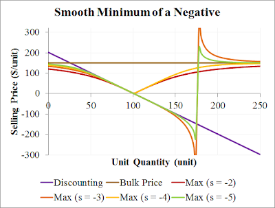
Before we attempt to deal with this issue, let's look at another interesting behaviour. Let's consider negative strengths. This chart shows strengths of -2, -3, -4 and -5:

A negative strength produces a smooth minimum function!

That's a convenient way to take the continuous minimum! And what happens when we feed in negative inputs? Well, it gets a little crazy:

A smooth minimum of a negative input does not look pretty.

So then, how might we deal with negative inputs? One way would be to transform inputs from the full number line onto just the positive half. To do that we turn to exponentiation. So here's the updated continuous maximum/minimum function, generalised to any number of functions: $$m(x, s) = \ln_b\left(\left[ \sum_{i=1}^q (b^{f_i(x)})^s \right]^{1/s}\right),$$ where \(b\) is the base of exponentiation. So, let's test it. I initially tried \(w = e\), but ran into overflow issues, and instead have used the value 1.01. Here is the maximum and minimum of positive and negative inputs, with \(s\) being 2, 5, -2 and -5:

A smooth minimum and maximum function that works with negative inputs.

One final thing. To use this in Lisp on individual values, evaluate this (with MathP):

(defun smooth-min-max (b s &rest vals)
    "Smooth minimum (s < -1) or maximum"
    #M log(reduce{#'+ vals :key fn(v) (b^v)^s}^(1/s) b))

And to construct a function that minimises or maximises other functions, try something like this:

(defun smooth-min-max-lambda (b s &rest funcs)
    "Returns a function that calculates a smooth min/max of the
given base and strength. If b > 1, positive s does maximisation,
negative s minimisation. If 0 < b < 1, it is reversed."
    (assert (or (< 0 b 1) (> b 1)))
    (assert (not (zerop s)))
    #M fn(&rest args) log(reduce(#'+ funcs :key fn(f) (b^apply(f args))^s)^(1/s) b))

Enjoy!

Analysis of Speed Density Flow Relationship

These notes have been inspired by a recent paper by Rahman, Ben-Edigbe and Hassan*. In it they analyse the speed, density and flow relationship.

The equations given in this previous traffic modeling post include an algebraic relationship between speed, density and flow: $$q=\rho v$$ and $$v = v_f(1-\rho/\rho_j),$$ where
\(q\) = flow rate (veh/s);
\(\rho\) = vehicle density (veh/m);
\(v\) = vehicle speed (m/s);
\(v_f\) = free flow speed (m/s), nominally 27.78 m/s;
\(\rho_j\) = jam density (veh/m), nominally 1/7 veh/m.

Given the above equations, it is possible to eliminate \(v\). That is, flow can be expressed in terms of density by using the speed equation:
$$q=v_f\rho ( 1 - \rho/\rho_j ).$$ This is a quadratic, and it has a maximum. Because it's a quadratic, this means that the inverse relationship is not a function, as it's multi-valued (one flow rate may be associated with two densities). Here is a graph of the flow-density relationship with the nominal values:

Relationship between flow and density, showing key values.

The maximum point on the flow curve happens to be the capacity of the roadway. We find the maximum point by differentiating the above and solving for slope equals zero. The critical density, \(\rho_c\) (the density at which the flow rate equals capacity), is found to be \(\rho_j/2\), and the capacity, \(q_c\), is given by:
$$q_c=v_f\rho_j/4.$$ With the values mentioned above (\(v_f\) = 27.78 and \(\rho_j\) = 1/7), the capacity is 0.99 veh/s, which while high, is in the right order of magnitude for freeways (which I think is around 0.5 to 0.7 veh/s).

The next post on this topic will be model discretisation.

* The paper is Rahman, R., Den-Edigbe, J. E., and Hassan A. (2012), Extent of Traffic Shockwave Velocity Propagations Induced by U-Turn Facility on Roadway Segments. 25th ARRB Conference. Mentioned here.

Macroscopic Model of Traffic

I work in the Intelligent Transport Systems (ITS) industry, at Transmax, and completed a PhD in applied mathematics at QUT. So it should come as no surprise that I want to combine and explore the two areas. To combine my two interests, I have investigated macroscopic models of traffic flow.

This post presents a simple model of traffic flow. It will form the baseline for further work and modifications. I learned of these equations from this paper by Paul Ross, published in 1988.

Model Equations

The first equation comes from the definitions of flow, density and speed:

$$q = \rho v,$$ where

\(q\) = traffic flow rate (veh/s) past the point;
\(\rho\) = vehicular density (veh/m); and
\(v\) = vehicle speed (m/s).

The above equation states that the number of vehicles that will pass by a point is equal to the density of traffic at that point times the speed of vehicles at that point. That is, flow rate increases with density and speed.

The second (partial differential) equation was given by Lighthill and Whitham in 1955. It describes the conservation of vehicles:
$$\frac{\partial \rho}{\partial t} + \frac{\partial q}{\partial x} = S(x,t),$$ where
\(\partial\) indicates partial differentiation;
\(t\) = time (s);
\(x\) = distance (m) along road; and
\(S\) = vehicles entering (+ve) or leaving (-ve) the road (veh/m/hr).

The third equation describes vehicle speed. The simplest relationship would have to be linear relationship between speed and density, as reported by Greenshields in 1934. This speed equation gives a free flow speed at zero density, and zero speed at the jam density:
$$v=v_f ( 1 - \rho/\rho_j )$$ where
\(v_f\) = free flow speed (m/s); and
\(\rho_j\) = jam density (veh/m), the average vehicles per metre in stationary traffic.

Let's say that the free flow speed is 100km/h. That means \(v_f = 27.78\) m/s. Also, let's assume that the average vehicle length is 5 metres, and that in a jam, they are spaced 2 metres apart. That means \(\rho_j = 1/7\) veh/m.

The equation for speed has an important effect on the traffic in the simulation, and has received a lot of attention in the literature. Various forms have been presented in the literature, and we will look at some of them in the future.

Boundary Conditions

A model with a partial differential equation is not complete without boundary conditions. There are a few options for us, but we must specify two boundary conditions - one for a point in space, and one for a point in time. First, some notation to help us specify the boundary conditions. We will refer to flow, density and speed as functions of two variables by writing \(q(x,t)\), \(\rho(x,t)\) and \(v(x,t)\).

Before we actually specify the boundary conditions, note that we have one partial differential equation, and two algebraic equations. With the two algebraic equations we can translate density to/from speed, and calculate flow from density or speed (but not the reverse - we'll see why below).

The time condition is usually chosen to be for time zero. We might choose that initially:
$$\rho(x,0) = 0$$ for all \(x\). In this model, it is equivalent to specifying \(v(x,0) = v_f\).

For this model, the space condition can be specified in terms of density or speed, as we can use the equations to determine the unspecified measures. Let's choose:
$$\rho(0,t) = \rho_j/4.$$ I don't think it's very important, but let's say that this condition overrides the time condition at \(x=t=0\).

In the future we may change the space condition to be a function of time, for example:
$$\rho(0,t) = \frac{(1+sin(2\pi t/T))}{2}\frac{\rho_j}{4}.$$

What's Next?

In another post we will analyse the relationship between speed, density and flow. After that we'll discretise the model equations so we can solve them numerically. And after that we may investigate the effect of different speed equations on model behaviour.

P.S. Thanks to MathJax and My technical memo for the script to render equations.

Window Peeler

I've said before that AutoHotkey is a great program that every Windows users should have and use. Here's yet another use I found for it to make my (and yours) life easier. Have you ever had two full-screen windows on the same monitor and wanted to switch between them quickly? I encounter that situation regularly. With two or three monitors, I use one in portrait orientation for email and viewing documents, and the others for everything else. To switch between windows, the Task Bar, Alt+Tab and Windows+Tab are great, but when I have 20+ windows open, it can take a fair bit of fiddling and time to switch between email and documents on the same monitor. I wanted a better solution. So I wrote this script (download):

;;;; Window Peeler - Show next window under mouse pointer
#NoEnv ;; Standard prelude
#SingleInstance force
SendMode Input
SetWorkingDir %A_ScriptDir%

;; Pick one of your mouse buttons (XButton1 = Back, XButton2 = Forward, MButton = middle button, LButton = left button, etc.) and use it here:
XButton1::
  MouseGetPos,,, WinId
  WinSet, Bottom,, ahk_id %WinId%
  ;MouseGetPos,,, WinId
  ;WinActivate, ahk_id %WinId%
Return

It moves the window under the cursor to the back when the back button is pressed on your mouse (assuming you have that button). That leaves the next window down on top! The two commented out lines of code activate that window, but I like it without that because it makes the script run quicker. It's a very simple script.

To make it trigger on another combination, for example Control+RightMouseButton, replace XButton1:: with ^RButton:: (^ is for Control).

P.S. Note that mouse software may interfere with the Back and Forward mouse button events. In the Logitech software, I had to set the action for that button to Other: Generic Button.

What do you think? Please leave a comment.

MathP is not CL Standards Compliant

Bad news! MathP, my very own mathematics notation library for Common Lisp, breaks the ANSI CL standard. The problem is that unread-char cannot be called consecutively without calling something that will read a character (like read-char). From the CL Hyperspec page for unread-char:

It is an error to invoke unread-char twice consecutively on the same stream without an intervening call to read-char (or some other input operation which implicitly reads characters) on that stream. 

I used it to basically peek multiple characters ahead, like peek-char, but for multiple characters. This may be why MathP doesn't work in CLISP. That allows me to have arbitrary operators. For example, I could have the following as distinct operators:

• * for multiplication
• ** (perhaps for exponentiation)
• .* (perhaps for element-wise multiplication, like in MATLAB)
• *. (dot product?)
• *.* (perhaps for element-wise exponentiation)
• etc.

I thought I was being clever, but such a use contravenes the standard pretty clearly. So I'm interested in alternatives. Does anyone know if it's possible to do multiple unread-chars with other stream implementations? Also, can you read lisp from them with standard reading functions?

Welcome to Seth Frederick Barton Johansen

Welcome to the world, Seth Frederick Barton Johansen! Seth is the son of Tamara and myself. He was born on the 3rd of November 2012, at 12:21 PM EST at the Wesley Hospital. He weighed 2728g (6 pounds), which is a bit small, but just fine. He also got a bit jaundiced (swallowing blood isn't good for you at that age).

 He's now 10 days old, and looking good:

Seth is a biblical name and means "Appointed". Seth was the son of Adam, and is an ancestor to Jesus. He replaced Abel, who was killed by Cain (Genesis 4:25).

He is a little bundle of joy. Good work Tamara (if you're reading this) - you did a great job growing him and giving birth to him - I'm very privileged to be married to you. Thanks Wesley Hospital for supporting Tamara and Seth through labour and the next few days, and to our heavenly father for his blessings, including our first son.

The heart of man plans his way, but the LORD establishes his steps. (Proverbs 16:9)

Also, thanks for the well wishes, hugs, flowers, and gifts everyone. They are lovely and appreciated.

P.S. The Wesley Hospital is a great place to have a baby - I can hardly recommend it highly enough. The staff were very friendly and helpful, and went beyond my expectations.

Some Random Windows Tips

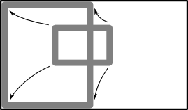
Having used Windows 7 for a while now, I an glad I discovered the Windows Button shortcuts. For me, they save a lot of fiddling with windows. For example, take the Windows+Arrows shortcuts. You may have noticed that it is possible to full-screen (maximise) a window by dragging it to the top of the screen, and to half-screen a window by dragging it to the side of the screen. But if you have multiple monitors, you'll notice that you can't half-screen a window by dragging to the edge of a monitor that abuts another monitor. Do not despair, it's still possible with the Windows+Arrows shortcuts! Here are the basics:

Half-screen a window by dragging it to the left, or pressing Windows+Left.

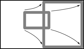
Moving in the other direction works as well:

Half-screen a window by dragging it to the right, or pressing Windows+Right.

To maximise a window, just press Windows+Up. If you have multiple monitors, you can 'hop' a window around by repeatedly pressing Windows+Left or Windows+Right combination:

Moving a window through all monitors and half-screen positions by repeatedly pressing Windows+Right (or Windows+Left).

Here are some more of my favourite Windows key combinations:

• Windows+D shows the desktop by minimising all windows (like Windows+M);
• Windows+E opens an explorer window;
• Windows+L locks the computer;
• Windows+Tab does a 3D version of Alt-Tabbing.

Many more shortcuts can be found here. While we're on the topic of Windows, here are some other tidbits:

• Ever had a window that is off-screen and you can't get it back? To get it back, activate the window from the Start Menu, and then press Alt+Space, then M, then press an arrow key (any will do), then move the mouse. I've used this trick since Windows XP to bring back rogue windows.
• To run a program quickly from the keyboard, just press the Windows key, then type in the first few letters of your program's name. If you type enough of the name for it to be the first choice in the Start menu, you can press enter to run it.

Got some favourite Windows shortcuts of your own? Let me know it the comments.

MathP and Macros

MathP and macros can be used together a fair bit. I've added a 'math-macro' capability to do custom parsing within MathP input, but you can write macros within MathP (as of version 1.11). I've added direct support for backquote (which has been tested in Corman Common Lisp). Here are some examples of how it all works:

Math-Macro

Macros that use structure in a way that conflicts with the mathematical notation of MathP (that's most macros) can define custom parsing rules. Here's the defun math-macro:
(define-math-macro 'defun (fn (maths)
        (multiple-value-bind (args todo) (parse-argument-list (cdr maths));; Skip name
            (push (car maths) *global-callables*);; Register the function (for recursion and later)
            (multiple-value-bind (body todo) (parse-assignment todo)
                (values `((defun ,(car maths) ,args ,@body)) todo)))))
The above shows that the defun math-macro parses the maths (after the defun symbol) as a name, an argument list and an assignment expression. So input maths of '(defun f (x y) x + y z) would be parsed to a list of one form: (defun f (x y) (+ x y)). The remaining maths (the second return value) would be '(z).

The above also shows how parsing is done in MathP. Note that maths is an argument to parsing functions (including the defun parsing function), and that parsing functions return two values. The first is a list of Lisp forms and the second is the maths remaining to be parsed.

But that's really only useful to give existing macros syntax. Let's dive deeper.

Backquote

As of MathP v1.1, it is now possible to use backquote (including nested backquotes etc.) in MathP. Backquote is used extensively in macro definitions, but can also be used outside of macros. We'll look at backquote first, to lay the foundation for MathP macros. Backquotes in Common Lisp are described in Section 2.4.6 of the Hyperspec. I've attempted to preserve it's behaviour but there are differences. First, a backquoted MathP expression gets wrapped in a progn if it needs it. One potential point of confusion is that in MathP, quote will quote list content without parsing it, but backquote parses content. Here are some examples of the similarities and differences:

#M'a[4]; expands to '(aref a 4)
and
#M`a[4]; expands to `(aref a 4)
#M'(1 2 3+4); expands to '(1 2 3 + 4)
but
#M`(1 2 3+4); expands to `(progn 1 2 (+ 3 4))

Backquote inside MathP

Firstly, a math-macro has been defined for defmacro. It has the same syntax as the defun math-macro. Here's a definition of aif like from On Lisp:
#Mdefmacro aif(test then &optional else) `(it=,test if it ,then ,else)

To include a documentation string, just put it and the body into brackets:
#M{defmacro aif(test then &optional else)
   {"Anaphoric if defined in MathP"
    `(it=,test if it ,then ,else)}}

It's also possible to nest backquotes, but writing a macro with nested backquotes is left as an exercise for the reader.

MathP inside Backquote (Backquote across Lisp and MathP)

I've found that the handling of backquote in Corman Common Lisp doesn't make it possible to consistently backquote a form in Lisp, and unquote something inside it from MathP. If you have a better result in another implementation, please leave a comment. For example (and please excuse the contrived-ness):


(defmacro make-more-func (number) `(lambda (n) #M n+,number))

Creating Bitmaps from Lisp

Having learned about programming computers later in my education (during university), the internals of computers and binary file formats have been very mysterious to me. Text files (and files with a text format) were usually understandable (or conceivably understandable), but binary files were impenetrable to me. At the time, I had no understanding of bytes, let alone concepts such as little/big-endianness. So, to get a feel for how binary file formats work, I wrote a bitmap writer function.

As reference, I used the Wikipedia page about the BMP file format. The code is released under a BSD license and is available for download here. It can make 24-bit colour bitmaps. It also contains some functions to manipulate colours. Bitmaps are created by calling a write-bmp function.

It was an interesting experience to work with binary streams, and I learned a lot. The code's not that nice, and probably not that efficient either, but it does what I want, which is output pictures.

One of the arguments to write-bmp is used to determine the colour of each pixel, and can be either a list of lists, or a function of two arguments. Here's a call that produces a twelve colour diagonal rainbow:
(write-bmp (path "bitmaps/diagonal-rainbow3.bmp") 80 80
  #'(lambda (row col) (rainbow12 (/ (+ row col) 2))))
The function rainbow12 selects a colour based on the floor of it's input mod 12. The above call produces*:

Here's a fun example using MathP:
(write-bmp (path "bitmaps/picture-perfect.bmp") 80 80
    #M(fn(r c)
       {applR = 2.5
        inRad(x y rad) = (c-x)^2 + (r-y)^2 < rad^2
        if inRad(15 65 6) yellow; inner sun
        if inRad(15 65 8) orange; outer sun
        if inRad(48 55 applR) || inRad(65 45 applR) || inRad(52 40 applR) red
        if (r-50)^2+(c-55)^2<15^2 darkgreen
        if r<20+3*cos(c/10) green; grass
        if 50<c<60 && r<50 brown blue}))
It produces*:

But since computers are good at calculations, let's try something a little more intense (and random, and ... psychedelic):
(write-bmp (path "bitmaps/trigonometric2.bmp")
    360 300
    #'(lambda (row col)
        (rainbow12
            #M{(row^1.1 + 0.6*col + 35*cos(col/15)*sin(row/16)
                + 2 * sqrt((row-250)^2 + (col-200)^2)
                + 20 * cos((col-0.3*row)/70) * (2-sin(row/80))
                + 20 * (1-cos(0.7+col/25)) * cos(0.6-row/50))/15})))
Viola*:

I hope your eyes aren't bleeding too much after that one. ;-)

I've also implemented some anti-aliasing, here's are some anti-aliased pictures:

The last one above is an attempt at creating a 'world' map with things like seas (blue), beaches (yellow), vegetation (green) and mountains (brown and white). The jump from vegetation to beach is sharp, but the anti-aliasing smooths it nicely.

* I've converted all of the pictures displayed here to PNG format using Paint.Net. It feels like cheating, but I was able to get things done. One of these days I'll look into ZPNG and Salza2. The compression used in the PNG format seems very mysterious to me.

I Am With You Always

Last Sunday I presented an exhortation at my church. The title is "I Am With You Always", and was inspired by the last recorded words of Jesus in the gospel of Matthew (28:18-20):

All authority in heaven and on earth has been given to me.

Go therefore and make disciples of all nations,

baptizing them in the name of the Father and of the Son and of the Holy Spirit,

teaching them to observe all that I have commanded you.

And behold, I am with you always, to the end of the age.

You can download my notes here. They're released under a Creative Commons Attribution 3.0 Unported licence. When I presented it, it took about 28 minutes.

I hope you find it an interesting read, and may God be with you.

Cody's Algorithm for ERF

Here's a more substantial example of the use of MathP. Erf(x) is the error function - a function related to the cumulative normal distribution. One way to compute the error function is with Cody's algorithm. I've implemented it in Common Lisp to double precision with MathP.

The implementation here starts by defining two constants (i.e. constants in the following equations), then three helper functions. The helper functions are the three rational functions denoted Rlm in Cody's paper. Here's the code in one big MathP expression:

#M{e = exp(1d0) irpi = 1/sqrt(pi); irp = inverse root pi
rlmErf(x) = (3.209377589138469472562d3;; The 4th degree polynomial from Table II.
      + x * (3.774852376853020208137d2
      + x * (1.138641541510501556495d2
      + x * (3.161123743870565596947d0
      + x *  1.857777061846031526730d\-1))))
      /     (2.844236833439170622273d3
      + x * (1.282616526077372275645d3
      + x * (2.440246379344441733056d2
      + x * (2.360129095234412093499d1 + x))))
rlmErc(x) = (1.23033935479799725272d3;; The 8th degree polynomial from Table III.
      + x * (2.05107837782607146532d3
      + x * (1.71204761263407058314d3
      + x * (8.81952221241769090411d2
      + x * (2.98635138197400131132d2
      + x * (6.61191906371416294775d1
      + x * (8.88314979438837594118d0
      + x * (5.64188496988670089180d\-1
      + x *  2.15311535474403846343d\-8))))))))
      /     (1.23033935480374942043d3
      + x * (3.43936767414372163696d3
      + x * (4.36261909014324715820d3
      + x * (3.29079923573345962678d3
      + x * (1.62138957456669018874d3
      + x * (5.37181101862009857509d2
      + x * (1.17693950891312499305d2
      + x * (1.57449261107098347253d1 + x))))))))
rlmEr2(x) = (-6.58749161529837803157d\-4;; The 5th degree polynomial from Table IV.
      + x * (-1.60837851487422766278d\-2
      + x * (-1.25781726111229246204d\-1
      + x * (-3.60344899949804439429d\-1
      + x * (-3.05326634961232344035d\-1
      + x *  -1.63153871373020978498d\-2)))))
      /     (2.33520497626869185443d\-3
      + x * (6.05183413124413191178d\-2
      + x * (5.27905102951428412248d\-1
      + x * (1.87295284992346047209d0
      + x * (2.56852019228982242072d0 + x)))))
defun erfc(x) {"Placeholder" x}
defun erf (x) {"Error function computed with Cody's algorithm"
    x = float(x pi); Make sure it's a double
    if x < 0.0 (-erf(-x))
    if x < 0.5 x * rlmErf(x^2)
               1d0 - erfc(x)}
defun erfc(x) {"Complementary error function computed with Cody's algorithm"
    x = float(x pi); Make sure it's a double
    if x < 0.5 1d0+erf(-x); Based on identities.
    if x < 4.0 e^-x^2 * rlmErc(x);; These two avoid subtraction from one.
               (oox2=1d0/x^2  e^-x^2/x * {irpi + oox2*rlmEr2(oox2)})}}

To check that it works, we have here a small selection of values for erf and erfc, sampled from the Wikipedia page, compared to those calculated using the above code:

erf(0.1) ≈ 0.1124629 ≈ 0.112463d0
erfc(15)/2 ≈ 3.6065e-100 ≈ 3.606497d-100
erf(0.95) ≈ 0.8208908 ≈ 0.820891d0
erfc(0.7) ≈ 0.3221988 ≈ 0.322199d0

Going a bit further, here are some values based on the arbitrarily precise values computed by Wolfram Alpha:

erf(1/100)
0.0112834155558496160
0.0112834155558496169...
erf(1/3)
0.3626481117660628000
0.3626481117660629334...
erf(1/2)
0.5204998778130465000
0.52049987781304653768...
erf(1)
0.8427007929497148000
0.8427007929497148693...
erf(4)
0.9999999845827421000
0.9999999845827420997...

So it appears (from this small sample at least) that this implementation is accurate to about 1e-16 (see the value for erf(1/3)), but usually 1e-17, which appears to be the resolution of doubles for Corman Common Lisp.

MathP is in git

Good news! The source code (and other tidbits) for my Common Lisp library MathP is available from my public git repository at bitbucket here. Please, go and fork as desired.

I've given MathP a logo at the same time:

Other logos I came up with and considered were:

Like a specific one? Let me know?

And since I want to show you more MathP, here's an implementation of exponential smoothing on the list of data points 0, 1, 2, 3 and 1:

#M{theta=0.2 d=nil
   s(x) = d := if !d x theta*x+(1-theta)*d
   mapcar(#'s '(0 1 2 3 1))}

It should produce the list:
(0 0.2 0.56 1.048 1.0384)

Simple Error Handling in Lisp

Yup, simple error handling in Lisp. Lisp has a really powerful condition/error handling system (also known as it's condition system). We won't delve into that here. This post was actually inspired by MS Excel (I use MS Excel a lot at work). There's an iferror function that may be used in spreadsheet formulae. It is entered into a cell like so:
=IFERROR(1/0, "failed")
In the above formula, because there is an divide by zero error in the first argument, iferror returns the second argument instead. It's simplicity means it's easy to use and understand.

To replicate this behaviour in Common Lisp is fairly easy. I've included it in MathP. Here's the definition as a macro:
(defmacro iferror (try fallback)
    `(handler-case ,try (error () ,fallback)))
Using it is just as easy as in Excel:
(iferror (/ 1 0) 'failed)
I hope the above code is useful to you; Use it however you want. I accept no responsibility for problems arising from it's use. If you do find it useful, I'd be tickled pink to hear from you.

Do you know of a similar macro? Please leave a comment.

If you use Windows, please use AutoHotkey

AutoHotkey is a powertool for Windows. It is one of my indispensable tools. I can hardly praise it highly enough. I use it for many things. I have used it to make using Windows less painful, and coding Lisp easier. Here are a few samples of AutoHotkey I use it to:

Make Caps Lock type hyphen (-) instead (I use hyphen a lot - you can make it do what you want):
SetCapsLockState, AlwaysOff
CapsLock::-

Swap brackets to my liking. Once I started programming Lisp, I quickly realised that round brackets should be easier to type. I've swapped ( and ) with [ and ]. I've also made the closing brackets get typed in when you type one of the opening brackets: (, [, or {. This one was the whole reason I started looking for something like AutoHotkey. Nothing else I've found can do this on Windows.
; The dollar signs stop the hotkeys from going into an infinite loop.
$[::Send (){left}
$]::Send )
$(::Send []{left}
$)::Send ]
$+[::Send +[+]{left}

Shorten some git workflow shortcuts (for example, typing gst then Enter is equivalent to typing git status then Enter):
SetTitleMatchMode 2
#IfWinActive, MINGW32:/
::gco::git checkout
::gcom::git checkout master
::gds::git diff --stat
::gdi::git diff
::gpu::git push -u
::gmm::git merge master
::gst::git status
::gct::git commit
::gcta::git commit -a

These and some other bits of AutoHotkey are packaged into a single script here.

I hope the above and linked script is useful to you; Use it however you want. I accept no responsibility for problems arising from it's use, but if you do find it useful, I'd be tickled pink to hear from you.

MathP Examples

MathP is my Maths DSL for Common Lisp. Here are some examples of it in use. If you want to run these examples, don't forget to either use MathP (use-package '#:mathp), or qualify uses of fn as mathp:fn. Here we go:

In simple calculations. The REPL becomes a very powerful calculator:
#M dt=6 v=9 nl=2 v/dt*3600d0/nl
I appreciate brackets, but I also find it a lot quicker to write these kind of expressions at the REPL.

Here's the choose function:
#M(defun choose (n k)
   {assert(integerp(n) && integerp(k) && n >= k >= 0)
    result = 1
    #L(loop for i from 1 to k do #M result *= (n-k+i) / i)
    result})
Note the use of logical and (&&) as well as chained comparisons in the assert expression. I've also used the mutating assignment operator *=. MathP also contains +=, -=, /=, ^=, &= and |= (the last two perform logical and/or, not bitwise and/or).

To calculate normal distributions with closures:
#M e = exp(1d0)  scale = 1/sqrt(2*pi) #L
(defun normal-distribution (mean stdev)
    #M fn(x) scale/stdev * e^-(0.5d0*(x-mean)^2/stdev^2))
In the above, we use #L to read in a lisp form from within the MathP form. The top level of the MathP form with the #L would normally stop reading at the end of the line, but the lisp reader invoked by #L conveniently consumes it for us.

And to test the above normal distribution calculator:
(loop with dist = (normal-distribution 0 1)
      for x from -3 to 3.1 by 0.2
    do (format t "~&~4,1F ~A~%" x
               (make-string (round #M 40 * #!dist(x))
                            :initial-element #\=)))
The #! above is a syntax for funcall, where the actual function call looks like a normal function call in MathP.

And one last one, the binomial probability mass function:
#M defun binomial (p n k) choose(n k) * p^k * (1-p)^(n-k)

MathP: Math notation in Common Lisp

MathP is my attempt at adding mathematical notation to Common Lisp.

Lisp has a beautiful, eminently grokkable syntax (if that even makes sense). It's great for general programming, macros and getting stuff done. Another of it's strengths is creating domain specific languages (DSLs). If you've tried to write more than basic mathematics in Lisp, you'll no doubt have wanted to write things like x+y*z or a*x^2 + b*x + c. I think many people who have just learned Lisp coming from other Algol style languages miss that expressiveness. They, like me, probably wanted a mathematics DSL. Well, now you've got one. MathP lets you write the above expressions within Common Lisp. MathP is a mathematics DSL.

MathP syntax attempts to retain a lot of the existing syntax of Common Lisp, while providing infix operators for mathematical notation. As a bonus, MathP syntax for function calls is vaguely similar to M-expressions, and there is a rudimentary macro system. More detail, including several examples, can be found in the documentation.

MathP is released under a BSD licence. It's been tested in Corman Common Lisp (on Windows).

[Edit: updated to version 1.1 - Support for backquote et. al.]
MathP Source Code
MathP Documentation (PDF) (original ODT)

To use it, download the source then load it with a call to load, something like this:
(load ".../path/to/MathP.lisp").

Here are some examples to try out (more can be found in the documentation and in the tests at the end of the code):

• #M area := length * width
• Positive root for a quadratic: #M x := (-b + sqrt(b^2 - 4*a*c)) / (2*a)
• Local function and shared syntax: #M f(x)=x^2+1 mapcar(#'f '(1 2 3 4))
• Factorial: #M defun fact(n) if n<=1 1 n*fact(n-1)
• Naive Choose: #M defun choose(n k) fact(n)/fact(k)/fact(n-k)
• Recursive Choose: #M defun choose(n k) {k=min(k n-k) prod(i res)=if i>0 prod(i-1 res*(n-k+i)/i) res  prod(k 1)}

Welcome to Metalight!

Welcome to Metalight. I will be posting some thoughts centred around programming (mostly with Common Lisp, but also AutoHotkey), mathematics, and God. I hope you enjoy, and find the coming posts interesting and informative.

I chose the name of this blog (Metalight, i.e. meta-light) because light is a great metaphor for understanding. If light is shed on a topic, it can be understood and obstacles may be navigated. If no light is shed on a topic, it is very difficult to understand, and when problems arise, it is hard to tell what the problems are. I want to shed light on these topics.

Whoever loves his brother abides in the light, and in him there is no cause for stumbling.

1 John 2:10

P.S. Please check out my links page.